Background (Why):
Openstack has component: Ceilometer (Telemetry). Ceilometer was huge and its main purpose was to help with the Monitoring and Metering of whole of th OpenStack. But because of the scale at which OpenStack operates, Ceilometer would often fall behind and become a major bottleneck for the same function it was designed to do. It had one more problem:- Aggregating these measurements and providing them in a more consumable format.
So it was broken into different parts and this gave rise to a time series database - Gnocchi.. Gnocchi stores data on the disk in its own custom format. And then using a group of processes on same node. On sharing the storage disk across different nodes, Gnocchi can form a cluster of processes from these nodes to aggregate the data. The received data is referred as metrics, as it is the measured usage of the various resources(like cpu, ram, disk, network) in OpenStack.
One of the ways Gnocchi is different is the way it handles aggregation. Instead of aggregating the metrics to generate (sum,mean,std-deviation etc) whenever and however they are asked for, Gnocchi makes the user choose on what kind of aggregations should be performed while defining the metrics and calculates and stores the metrics and aggregates immediately on receipt.
So the user has to tell Gnocchi that the metrics X should be received at interval A but should be also aggregated to interval B to make Y aggregates and then data should be archived after N time.
For example:
Receive cpu-usage-vm every 5 sec and generate sum,mean,std-deviation for 1m, 10m, 30m, 1h, 12h, 24h, 7d, 15d, 30d, delete after 30days.
As the received data are immediately aggregated and stored, retrieval is as good as a single disk read. In a way the aggregation problem (as faced by ceilometer, as mentioned above) is never faced and so does not needs solving. But this pre-computing was still a problem as the amount of data could get really overwhelming. Gnocchi tries to solve this problem by letting a large number of worker aggregate the data forming a cluster over distributed nodes.
This peculiar way of restricting the problem space and commitment of the range of values for the variables involved in aggregations allowed some space for Experiments.
Speeding up (How)
The workers working across different nodes have their work partitioned at run time.
- Input size for metrics to be aggregated is already known
- The aggregation intervals are already defined along with the metric
If one knows there are X points at A intervals to be aggregated to generate Y points at B intervals then this forms a classic case of Parallelization, where you can employ Y threads to aggregate (X/Y) points from X, as shown in the following figure.
 |
 |
|---|---|
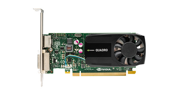
| Reduction example from devblogs.nvidia.com | Quadro K620 (Image from Nvidia.com) |
Now there are various ways one could implement this parallelization in the form of threads by offloading it to the cores of the CPU. But the poor CPU is already busy juggling processes and there is always some process fighting for the CPU’s attentions. Also the CPU has only so many cores, so the idea was to use a GPGPU to get the massive parallelism required.
So for this experiment I decided to leverage the GPU my machine was already equipped with, an NVDIA Quadro K620.
The specs of the GPU can be seen here. It is a medium-grade GPU, with good compute capability (5.0) and 2GB of ram.
Implementation (is it even possible-?)
The first approach was to get at least the benchmark passing and with a speed up.
The benchmark covered a wide range of data formats and multiple areas of the carbonara library. It has (De-)Serialization evaluations, resampling and aggregations (sum,min,max,mean,average), and in addition the input data for all these benchmark evaluation was not just arrays of random values, but arrays of zeros, random floats between in the range [-1,1]. So
the requirements was to beat all these benchmarks.
First step was to insert a class in carbonara library (my copy) which could call the CUDA code, and simulate addition with a fixed re-sample rate(30s) and fixed input size for all zeros and continuous numbers as floats.
This itself gave a performance boost. From here on the game was to increase performance and throughput while keeping the semantics intact.
Getting the initial kernel going was easy. There was already a speed-up of 5x.
The first bottleneck was the amount of data processed in one go. The benchmark assumed an input size of 3600 points for calculation. This number was very low. Reducing 3600 points to 600 points in parallel on a GPU would in the naive implementation about 600 threads (6 aggregates each). As recent GPGPUs generally have a compute capability > 5. This allows a block to contain a maximum of 2048 threads so 600 was very small, and thus was increased to 1024 * 1024 * 6
There is one more reason for the number to be so high. Since the GPU has its own memory input data needs copying from HtoD (host to device i.e. CPU-RAM to GPU-RAM). But even this device memory is not fast enough. Every access to load data (from device memory to L2 cache) for computation is expensive, so to hide the latency lots of computation is recommend. So that while data is loading, any already loaded data can be used for computation. This is just one the ways to hide that latency.
In the part 2 I will start with a basic kernel (the piece of CUDA code that executes on GPU), perform some profiling with nvprof and visual profiler and apply optimizations to remove the bottlenecks. In part 3 some learning and further GPU-fication of other parts of the library.